Penalizing Complexity

“With four parameters you can fit an elephant to a curve; with five you can make him wiggle his trunk.”

–John Von Neumann

Models are simplified representations of the world around us. Sometimes by simplifying something, we’re able to see connections that we wouldn’t be able to notice with all the messy details still present. Because models can represent relationships, they can also be used to predict the future. However, sometimes modeling something too closely becomes a problem. After all, a model should be a simplified version of reality: when you try to create an over-complicated model, you might begin noticing connections that don’t actually exist! In this blog post I’ll discuss how regularization can be used to make sure our models reflect reality in meaningful ways.

Overview

Regularization is a topic that’s often applied in machine learning. Regularization reduces the complexity of a model by penalizing the magnitude of its coefficients. But what are a model’s coefficients? And how does “penalizing” help us get better results? In the next few sections, I’ll show how linear regression can be used to fit some data. After that I’ll show you that it can be problematic when a model fits the data too well. Then I’ll introduce different ways of talking about distance and finally show how this can be used to improve a model.

Linear Regression

Consider the affine equation \(y = \beta_0 + \beta_1x\). This is known as the equation of a line and was probably presented to you in middle school under the guise of \(y = mx + b\). We can use this to model a linear relationship between variables (an input variable, \(x\), and an output variable, \(y\)) along with \(\beta_0\) and \(beta_1x\) which are just numbers that make our equation work. The equation of the line is defined by two variables \(\beta_0\) (the y-intercept) and \(\beta_1\) (the slope of the line). But how do we find these values?

It makes sense to start off by defining what the best line should do: it should minimize the difference between each data point and the line. For instance, when you plug a value for \(x\) into the equation, the difference between the actual corresponding y-value and the y-value predicted by the model (often written \(y'\)) is your error. Of the two lines below, the green line does a much better job of modeling our data than the red line (notice also that the data above was divided into a training set and a test set. In the next section I’ll justify why this division was made):

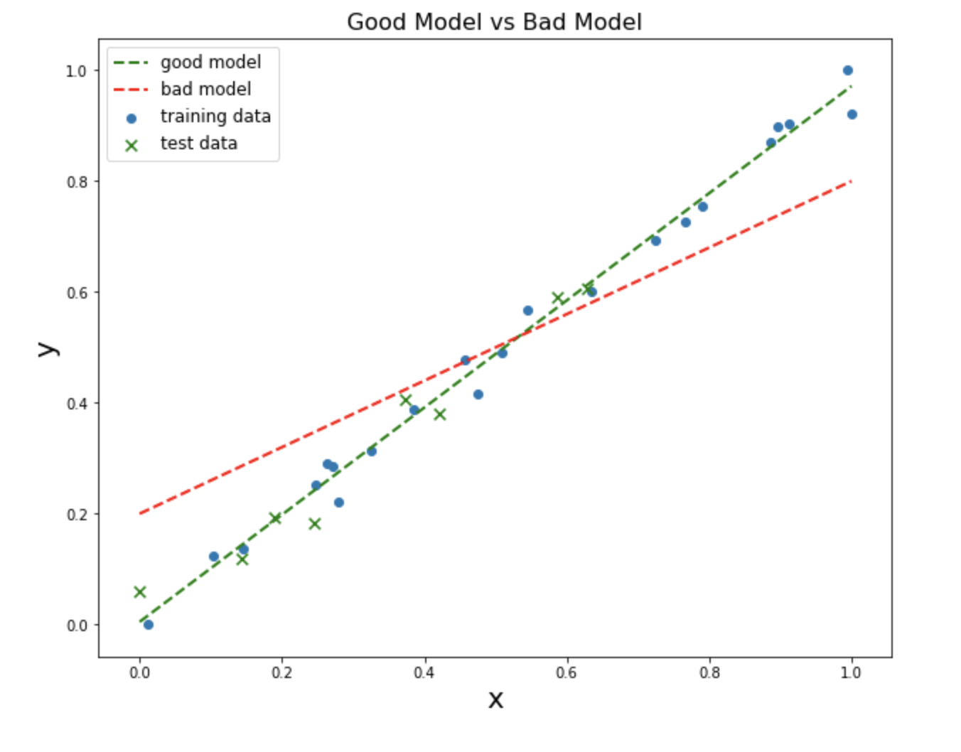
You can imagine summing up all the errors to obtain the total error of the model (actually, you sum the squared error). The predictions of a linear regression model will always lie on a line. The best model will minimize the sum of squared errors (where \(y'\) is the predicted weight and \(y\) is the actual weight for a given height. \(n\) is the total number of data points in your possession).

This can be written even more explicitly as:

The mean squared error (MSE) is the total error divided by the number of data points. MSE is a measureemnt commonly used in machine learning. The MSE for the green line’s training set is 0.002, whereas it’s much higher for the red line: 0.009

One approach to finding the line of best fit would be to create lots of random lines and calculate the sum of squared error between each line and the data. The line with the lowest error would be the model that you choose. (Note: the model is not actually generating a “line” – the model generates points which all fall on the same line.)

However, this is an inefficient way of doing things. You could imagine tweaking the values of the coefficients in a more intelligent way, so that they eventually settle onto a reasonable solution that’s guaranteed to be the best. We can use gradient descent to assign a fraction of the squared error to each coefficient. Gradient descent tells us which way the coefficient needs to be tweaked, and we can tweak it in that direction over many epochs until the error is it a minimum. A formal explanation of gradient descent is beyond the scope of this blog post.

In the sort of models that get used in the field of deep learning, we have to use optimization techniques like stochastic gradient descent to find the best (or much more often, “the most acceptable”) values for the coefficients of our model. Luckily, we don’t have to go down this pathway when dealing with linear regression. There is a closed-form solution that will always give us the best answer for our coefficients. In the next section I’ll show how models can fit data too-closely and how we can prevent this.

Complexity

The parts of a model that a machine learning algorithm tries to learn are the coefficients (\(\beta_0\) and \(\beta_1\) above). More complicated models have more coefficients (also called parameters). A model with more parameters is able to learn to represent more complicated data (for instance, it would be unrealistic to assume that people recognize faces based on only two parameters: let’s say \(\beta_0\) is pupil-separation and \(\beta_1\) is nose size – there are probably hundreds of things that differentiate one face from another.)

Deep learning models are able to learn amazing things, but there is often a cost to this complexity. A model with lots of parameters that are allowed to fluctuate wildly can overfit the training data. For instance, we can create a very complicated high-degree polynomial model that very-closely fits the above data:

This model has MSE that’s even lower than the “green” model above: 0.0003. But it’s unlikely to generalize to any new data that we receive:

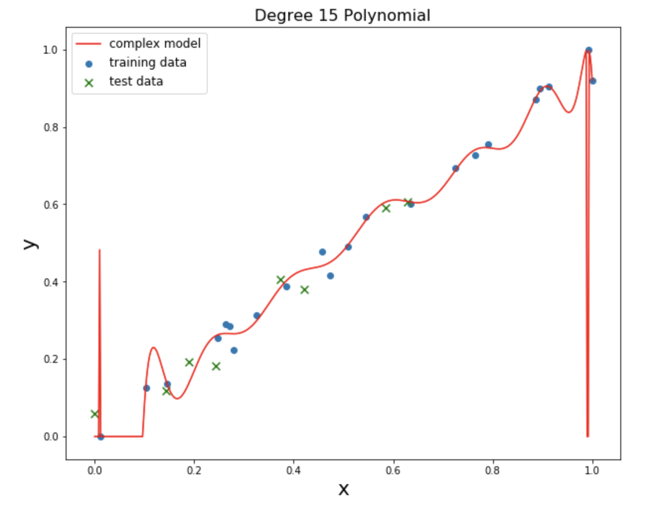
The way that we can prove that a model is unlikely to generalize to new data is by applying a model that was fit to a training set and try it out on our test set. Although the polynomial model’s MSE for it’s training set is only 0.0003, it’s MSE for its test set is 14.24. Compare that with the numbers for our “green” model: training = 0.002 and test = 0.0015. The green model is much more likely to perform well on new data than the polynomial model.

But let’s say that we’ve been given a model like the one above: a polynomial model with 15 different coefficients we can tweak. At first it might seem like there will always be too much flexibility: the model will just fit any training set, meaning it’ll fail on the test set. One way to get around this is with regularization.

Regularization

A complex model is a model with lots of coefficients to fit. Regularization is the process by which we simplify a model by reducing the impact of some of its coefficients. For instance, a model like \(y = \beta_0 + \beta_1x + \beta_2x^2\) is more complex than \(y = \beta_0 + \beta_1x\) because the former has more coefficients to fit. We can penalize large values for the coefficients by adding the value of the coefficients to the loss function we’re using (\(\lambda\) is a parameter that controls the amount of regularization):

This is one way to penalize large coefficients. A similar method is to add the squared coefficients:

These two methods are called lasso regression and ridge regression, respectively. And the only difference between the two is how distance is measured. When we try to minimize our error, we longer just care about the MSE – we’re also adding the regularization term.

Here is the same degree-15 polynomial but with regularization applied to it:

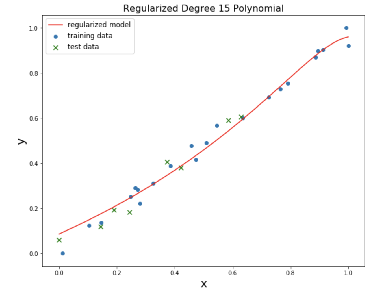
Ridge and lasso regression behave differently: ridge tends to shrink all of the coefficients at the same time, whereas lasso tends to shrink some of the irrelevant coefficients all the way to 0. To demonstrate why this is the case, it’s important to talk about how to calculate distance.

Distance

The most obvious way to talk about the distance between two things is the Euclidean distance, where the distance between two points in space is the straight line that connects them. If we have some vectors \(\mathbf{a}, \mathbf{b} \in \mathbb{R}^2\) that represent points in 2-D space, then the Euclidean distance between vectors is:

This makes intuitive sense, and is intimately related to the Pythagorean theorem: the distance between the vectors is like finding the hypoteneuse of the right triangle that defines the common \(x\) and \(y\) components of the vectors.

But this isn’t the only way to think about distance. If you try to get from the Mission up to SOMA, you’ll find yourself traveling at right angles, following the city blocks. In cities, Euclidean distance doesn’t make sense. Instead you can find the Manhattan Distance between points:

A norm is a function that takes in a vactor and returns a positive number, representing the distance between that vector and the origin. The \(L_2\) norm is:

Notice that this is almost exactly the same as the formula for Euclidean distance. In fact, is is the same formula, except that it’s measuring the distance between each component, \(x_i\), of the vector \(x\) and the origin: the origin is \(0\) everywhere, and it’s not necessary to represent \(x_i - 0\) in the formula. If we wanted to use the \(L_2\) norm to measure the Euclidean distance between two vectors, we would subtract all of the corresponding elements before squaring them, and would get the Euclidean distance formula. The Manhattan norm is called \(L_1\) and other norms are defined. The \(L_p\) norm is just:

Let’s say that we have a vector \(\mathbf{x} = [3, 4]\). The \(L_2\) norm is \(5\) (remember your 3:4:5 triangles from Elementary School!). The other norms are:

Notice that these numbers are converging towards \(4\), the largest element of the vector \(\mathbf{x} = [3, 4]\). The \(L_{\infty}\) norm is just \(max(\mathbf{x})\).

So why does lasso regression, which uses the \(L_1\) norm shrink some coefficients to 0, whereas ridge tends to shrink things more equally? If the elements in your vectors represent coefficients, and the norm of the vector is added to your loss function as its regularization term, then consider the effect of reducing elements to 0 under different norms:

Under \(L_1\) the effect of reducing the first element of the vector to 0 changed the norm from 7 to 4 – a big difference! The difference under \(L_2\) is smaller:

This is the reason why the different regularization don’t behave the same way: they’re measuring distance in different ways!

Putting it all Together

It’s important to constrain the complexity of our models. We don’t want our models to fit our data too closely, or they’ll begin to lose some of the predictive power we value. The principle of Occam’s Razor says that when two models describe reality equally well, we should go with the simpler one. Regularization is one way of enforcing this principle. Different regularization techniques apply regularization differently, and this is because of how they measure the distance between things.

See the corresponding notebook for more detailss.