Math to Code

When I’m trying to decipher some hairy math formula, I find it helpful to translate the equation into code. In my experience, it’s often easier to follow the logical flow of a programming function than an equivalent function written in mathematical notation. This guide is intended for programmers who want to gain a deeper understanding of both mathematical notations and concepts. I decided to use Python as it’s closer to pseudo-code than any other language I’m familiar with.

This is not meant to be a reference manual or encyclopedia. Instead, this document is intended to give a general overview of mathematical concepts and their relationship with code. All code snippets were typed into the interpreter, so I am omitting the canonical >>>.

Table of Contents

1. Sequences
   • Finite Sequences
   • Infinite Sequences
2. Series
   • Series Summation
   • Series Product
3. Sets
   • Union
   • Intersection
   • Difference
   • Complement
   • Ordered n-Tuple
   • Cartesian Product
4. Logic
   • Universal Quantifier
   • Existential Quantifier
   • Implication
   • Biconditional
   • Negation
   • De Morgan’s Theorem
5. Calculus
   • Integrals
   • Gradients

Sequences

Finite Sequences

A finite sequence is also called an n-tuple, where n is the length of the tuple:

The elements of a sequence can repeat and can be of any data type. Order is important in a sequence, and every element has an index. This is similar to a list in Python:

A = [1, 5, 10, 25, 50]

Because a sequence is ordered, every element in the sequence has an index. For instance, the second element of the list is \(a_2\), which is the same as A[1] in Python (remember, elements are indexed differently in math and computer science).

Let’s say that we want to sum every element in a sequence:

To do this, we count from 1 to n, where 1 is the first list index and n is the final list index (=5).

The length of a sequence is also called its cardinality, which is often written as:

And is equivalent to:

len(A)

Infinite Sequences

An example of an infinite sequence are the odd numbers:

It’s often more useful to specify a function that generates an infinite sequence than simply implying a function using \(...\) (more on that at the end of this section):

An infinite sequence is analogous to a stream in computer science. In Python, generators exhibit streaming behavior and can imitate the behavior of an infinite sequence. Unlike lists, generators do not store a collection of values. Instead, they generate their values only when needed. Because a computer’s memory is not infinite, a list can never imitate the behavior of an infinite set. The generator below produces odd numbers:

def odd_numbers():
    i = 1
    while True:
        yield i
        i += 2

In math, infinite sequences and series also have cardinality. For instance, the cardinality of the natural numbers is \(\aleph_0\) and the cardinality of the real numbers is \(\mathfrak{c}\). One of Georg Cantor’s surprising discoveries was that the set of all positive odd numbers has the same cardinality as natural numbers (intuitively, it seems like there are twice as many natural numbers as there are odd numbers). This is because infinite sets are not measured by counting their elements – after all, that would be futile, because you’d go on counting forever. Instead, infinite sets are measured by the functions that generate them. If a function can be lined-up 1:1 with the natural numbers, then it has the same cardinality as the natural numbers, \(\aleph_0\), and is called “countably infinite”. There are some sets that are uncountably infinite (more on that in a second).

Given a generator that produces the natural numbers, we can create a second function that gives us the odd numbers by chaining them together, demonstrating that these sets have the same cardinality:

def natural_numbers():
    i = 1
    while True:
        yield i
        i += 1

def odds():
    for k in natural_numbers():
        yield 2 * k + 1

# if we iterate through odds(), we get odd numbers
for i in odds():
    print(i)

However, we cannot use our natural number generator to produce the set of real numbers. Think about it. Let’s say that we start counting from 1. What is the first real number that comes after 1? It’s got to be something very close to 1, like 1.01. Well, this isn’t close enough, because 1.0001 is even closer. In fact, we can keep adding 0’s and never stop (well, actually, our computer will eventually run out of memory and crash).

I’m not a professional mathematician, but my failure to think of a function that gives us the real numbers seems to be evidence that the cardinality of the real numbers is strictly greater than the cardinality of the natural numbers. Apart from a before-the-fact specification of our accuracy (e.g., limiting numbers to 100 digits), it seems like this problem is intractable. In other words, you can translate countably infinite sequences from math to programming, but uncountable sets are trickier.

(If anyone has any insight into this problem, please send me an email, as I’m very curious to hear more.)

Series

Series Summation

Sigma Σ represents summation:

Because Python is indexed from 0, in order to count from 1 to n, we count from 1 to n + 1:

total = 0
for i in range(1, 11):
    total += 2 * i

Sums can also be linked together. When both sums are finite, order doesn’t matter. This is extremely close to the idea of a for loop:

Sums are evaluated from right to left. This means that the left-most sigma is the top-most nested loop:

total = 0
for i in range(1, 5):
    for j in range(1, 3):
        total += i * j**2

Series Product

The product of a series is represented by a capital letter pi Π:

This is similar to the code for summation, except that we initialize the total at one and multiply it by the expression currently being evaluated:

total = 1
for i in range(1, 5):
    total *= i

Notice that this particular instance of summation is equal to \(4!\)

Sets

Union

Given a set A and a set B, the union of A and B is the set of items from either or both sets:

The direct equivalent in Python is:

A = {1, 2, 3, 10, 11}
B = {1, 3, 7, 9}
A | B # {1, 2, 3, 7, 9, 10, 11}

However, the above examples obscure union’s relationship to logical OR:

Intersection

The intersection of two sets is the set of items that belong to both sets. Using A and B from above:

The Python equivalent is:

A & B # {1, 3}

The set intersection is related to logical AND:

Which in Python is:

{i for i in A if i in B} # {1, 3}

Difference

The difference between set A = {1, 2, 3, 10, 11} and set B = {1, 3, 7, 9} are the items in A that are not in B:

The syntax in Python is very close to the set syntax:

A - B # {2, 10, 11}

This can be expressed more verbosely as:

Which is equivalent to:

{i for i in A if i not in B} # {2, 10, 11}

Complement

The complement of A is everything in the universe, U, that is not in A. In our case, the universe will consist of \(U = \{1, 2, 3, 4\}\), where \(A = \{1, 3\}\):

Let’s pretend that we don’t know what the universe consists of, but instead we have access to sets which represent samples from that universe. Let those sets be A (above), \(B = \{1, 2\}\) and \(C = \{4\}\). The union of all those sets gets us as close to understanding the entire universe as we can get: \(A \cup B \cup C = \{1, 2, 3, 4\}\).

Assuming we have these sets set up in Python:

U = A | B | C
complement_A = U - A # {2, 4}

Ordered n-Tuple

An ordered n-tuple \(<x_1, x_2, x_3, ... x_n>\) is equivalent to a list in Python with n elements.

Cartesian Product

For sets A and B, the Cartesian product is the set of all ordered pairs \((a, b)\) where \(a \in A\) and \(b \in B\). In set-builder notation, this is:

Let’s say that \(A = \{a_1, a_2, a_3\}\) and \(B = \{b_1, b_2\}\), then \(A \times B\) is:

In Python, this is:

A = {'a1', 'a2', 'a3'}
B = {'b1', 'b2'}
{(a, b) for a in A for b in B} # {('a2', 'b2'), ('a3', 'b2'), ('a1', 'b2'), ('a1', 'b1'), ('a2', 'b1'), ('a3', 'b1')}

Logic

Many of the symbols in logic are similar to those used when we talk about sets. For instance, set intersection, \(\cap\), is similar to the logical conjunction \(\wedge\) (AND). And set union, \(\cup\) is similar to the logical disjunction, \(\vee\) (OR). These logical connectives are similar to what you see in sets.

Universal Quantifier

The universal quantifier, \(\forall\), means “for all.” For instance, this formula:

When Q(x) is the statement “x is less than 50,” this statement evaluates to True. If, on the other hand, Q(x) was “x is an odd number,” this statement would be false, as 2 and 4 are not odd numbers.

This has a simple implementation in Python:

A = {1,2,3,4,5}
def Q(i):
    assert i < 50

for i in A:
    Q(i) # nothing returns

But what if we change Q?

def Q(i):
    # tests if the number is odd
    assert (i - 1) % 2 == 0

Now we get an AssertionError, indicating that the statement evaluates to False.

Existential Quantifier

The existential quantifier symbol, \(\), means “there exists.” For instance, the formula below means that there exists one number in the set \(A\) such that condition \(Q\) is met:

For instance, if \(Q(x)\) is the statement \(x^2 = 25\), then this is evidently true, as \(5 \times 5 = 25\).

The Python translation of this would be to create a function, Q, that immediately returns true if it encounters any element that meets its criteria, otherwise it returns false:

A = {1,2,3,4,5}

def Q(li):
    for i in li:
        if i**2 == 25:
            return True
    return False
Q(A) # True

Implication

Arrows are used for implication. For the material implication (below), if A is true, then B is true too:

The Pythonic version of this is quite simple:

A, B = True, True
if A:
    assert B

A, B = True, False
if A:
    assert B # AssertionError

Biconditional

An arrow with two heads is the biconditional. \(A \iff B\) means “A is true if and only if B is true.” This is often written as “A iff B.” The biconditional is equivalent to \((A \Rightarrow B) \cap (B \Rightarrow A)\).

In code, this would mean that before we evaluate A, we first need to check B:

def biconditional(A, B):
    A = False
    if B == True:
        A = True
    return A

This function takes two arguments, A and B. A is returned as true if and only if B is true. This is done by first setting A to False before evaluating it.

Negation

\(\neg A\) means “not A” and is true only when A is false. This is easily understood in the context of an if-then statement:

A = False
if not A:
    print('A was false') # A was false

Logical negation is similar to the set operation complement.

De Morgan’s Theorem

De Morgan’s Theorem relates the concepts of conjunction and disjunction (similar to union and intersection, respectively) with negation:

and

Logical negation is similar to the idea of a complement from set theory. If we consider the first statement, this means “everything not in A or B is equal to the intersection of everything not in A and everything not in B.” If we have a universe, \(U\), and two sets, \(A\) and \(B\), we can represent this in Python using the set operations listed in the Sets section:

U = {1,2,3,4,5,6,7,8,9}
A = {1,2,3}
B = {3,4,5}
(U - A & U - B) == U - (A | B) # True
U - (A | B) # {8, 9, 6, 7}

Calculus

Integrals

Suppose we have a function, \(f(x) = sin(x)\). The area under \(f(x)\) from 0 to \(\pi\) is represented by the blue region in this graph:

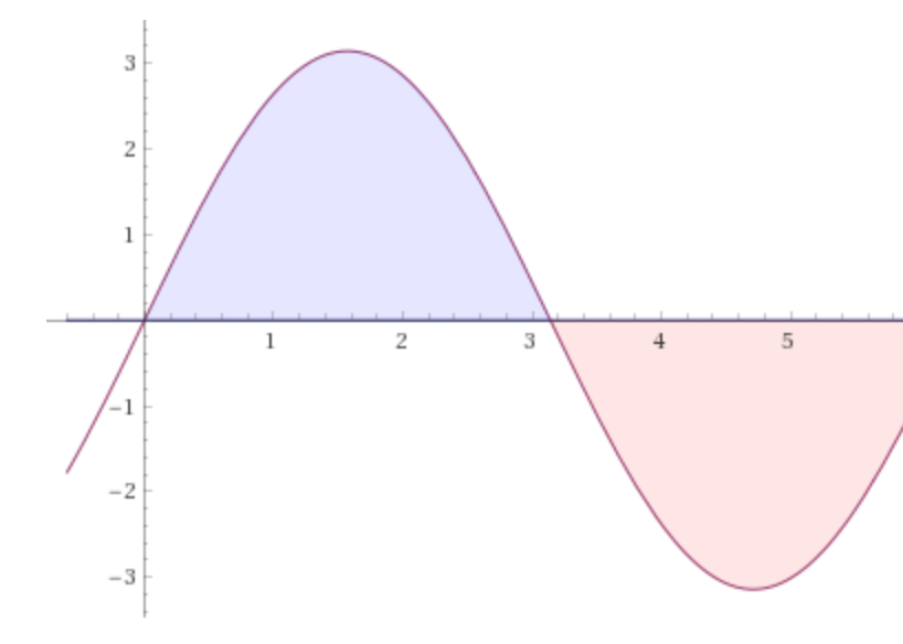
Which can be written as an integral:

Integration in Python is simple:

import scipy.integrate as integrate
from numpy import sin
pi = 3.14159
integrate.quad(lambda x: sin(x), 0, pi)
# (1.9999999999964795, 2.2204460492464044e-14)

In the tuple that gets returned, the first value is the integral and the second value is the upper bound on the possible error.

But what if we want to know the area under a graph with more than one dimension, like \(f(x, y) = sin(x) sin(y)\)?

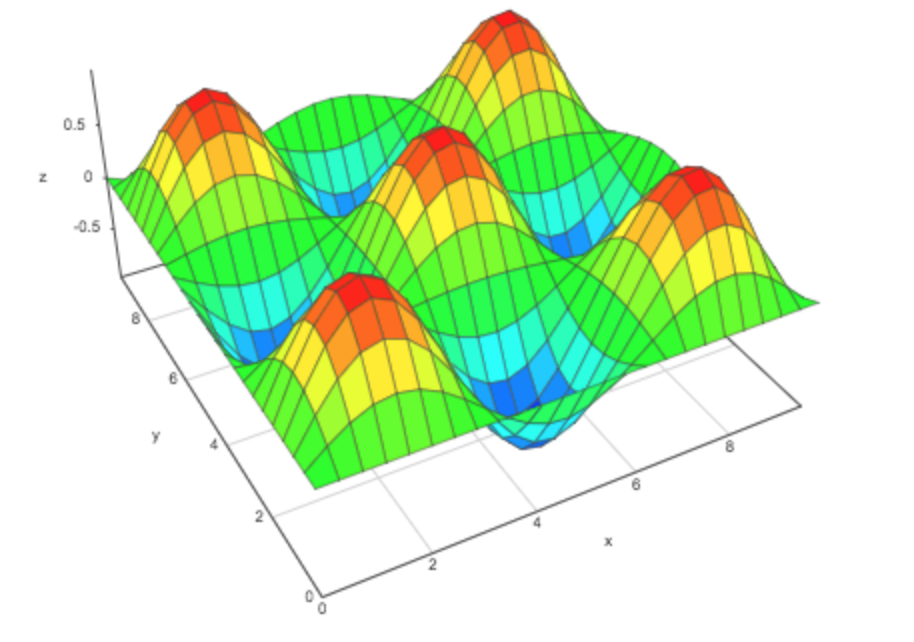
Let’s say that we want to know the area under the curve of 0 to \(pi\) on the y-axis and 0 to \(pi\) on the x-axis. The solution is to take a double integral:

In Python, you can use scipy’s dblquad function. This takes as arguments a function to be integrated, a pair of bounds for the outer integral, and a pair of inner bounds wrapped in functions for the inner integral:

from scipy.integrate import dblquad
def sines(x, y):
    return sin(x)*sin(y)
dblquad(lambda t, x: sines(t, x), 0, pi, lambda x: 0, lambda x: pi)
# (3.9999999999859175, 4.4408920984849916e-14)

Gradients

I’m not going to cover single-valued derivatives here, because they’re too simple. But what if you want to find the derivative of a vector-valued function with more than one argument? The gradient evaluated at a given point gives you some idea of a function’s multivariable slope at that point. A gradient is a vector of a the partial derivatives of a function. Gradients are important in some Machine Learning algorithms. The gradient of a function, \(f\), is written as \(\nabla f\). The symbol \(\nabla\) is called “nabla” or “del.”

If we have a function \(f(x, y) = x^2 - xy\), then:

I recommend using the Python library Theano for gradient operations:

import numpy
import theano
import theano.tensor as T

x = T.dscalar('x')
y = T.dscalar('y')
z = x**2 - (x * y)
gy = T.grad(z, [x, y])
f = theano.function([x, y], gy)
# test out a value
f(1, 0) # [array(2.0), array(-1.0)]

This is congruent with the result: